The figure below shows the steps in order to find the \$K_{cr}\$(or \$K_u\$) and \$P_{cr}\$ (or \$P_u)\$, by changing the proportional gain only (with \$T_d=0\$ and \$T_i=\infty\$) - an example for temperature control:

The time unit to be used should be consistent with its response curve. The relationship with the sample period \$\Delta t\$ can be obtained, after the discretization of the PID controller. Using the standard form, in contrast with other implementations (for example, when the derivative term is taken from output):
$$u(t)=K_pe(t)+\frac{K_p}{T_i}\int_0^t{e(\tau)d\tau+K_pT_d\frac{de(t)}{dt}}$$
Taking the derivative of \$u(t)\$:
$$u'(t)=K_pe'(t)+\frac{K_p}{T_i}e(t)+K_pT_de''(t)$$
A possible approach: To approximate the first and second derivatives using finite differences (eg backward), where \$k\$ is the sample id:
$$x'(t)\approx\frac{x_k-x_{k-1}}{\Delta t}$$
$$x''(t)\approx\frac{x_k-2x_{k-1}+x_{k-2}}{\Delta t^2}$$
So, the discrete PID controller takes the form (velocity algorithm):
$$u_k=u_{k-1}+K_p[(1+\frac{\Delta t}{T_i}+\frac{T_d}{\Delta t})e_k+(-1-\frac{2T_d}{\Delta t})e_{k-1}+\frac{T_d}{\Delta t}e_{k-2}]$$
Alternative definitions can include \$K_i=\frac{K_p}{T_i}\$ and \$K_d=K_pT_d\$. Also, the derivative term can be modified in order to reduce issues with high frequency noise - eg a low pass filter. Other discretization methods exist as well, such as Tustin, ZOH.
FURTHER EXPLANATION:
- Choose a sample time \$\Delta t\$ consistent with your process. There is extensive literature on the subject. For example, to avoid aliasing \$F_S > 2F_{BW}\$. In practice: Sampling frequency should be 10 to 30 times the bandwidth freq.
Set \$K_p\$ to some low value (with \$T_i=\infty\$ and \$T_d=0\$ at this stage). So, the above equation is simplified to:
$$u_k=u_{k-1}+K_p(e_k-e_{k-1})$$
Implement the previous equation (a P controller) in your digital system along with that suitable \$\Delta t\$, testing \$K_p\$ to see if it causes continuum oscillation (marginally stable). If the oscillations decay, keep increasing \$K_p\$. If the oscillations increase in amplitude (unstable system), reduce \$K_p\$. Do this until the system is marginally stable. When you arrive at this point, you have found \$K_{cr}=K_p\$ and \$P_{cr}=\$oscillation period (see the figure above).
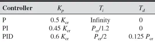
Using the table you have provided (also above), determine the \$K_p\$, \$T_i\$ and \$T_d\$ values from the \$K_{cr}\$ and \$P_{cr}\$ ones.
Implement the complete PID controller:
$$u_k=u_{k-1}+K_p[(1+\frac{\Delta t}{T_i}+\frac{T_d}{\Delta t})e_k+(-1-\frac{2T_d}{\Delta t})e_{k-1}+\frac{T_d}{\Delta t}e_{k-2}]$$