0

I have an open-loop transfer function G

num=105*conv([1 1],[1 2 43.25]);

den=conv([2 0 0],conv([1 2 82],[1 2 101]));

G=tf(num,den);

and a closed-loop function of G/(1+G). Here are the open-loop bode diagram and closed-loop bode diagram for that transfer function.

This is the open loop bode plot : bode(G)

enter image description here

This is the close loop bode plot:bode(G/(1+G))

enter image description here

We can see that for the open-loop function, the phase of the low frequency is almost inverted, meaning that self-excited oscillations are caused. But for the closed-loop function, the low-frequency phase is 0, meaning that the system is safe. So in this case, does the phase margin indicator fail?

zymaster
  • 19
  • 6

2 Answers2

1

So in this case, does the phase margin indicator fail?

Yes; due to the peculiarity of the system being considered.

I couldn't locate a straight text book reference. This is close enough.

From Wikipedia (emphasis mine)

This criterion is sufficient to predict stability only for amplifiers satisfying some restrictions on their pole and zero positions (minimum phase systems). Although these restrictions usually are met, if they are not another method must be used, such as the Nyquist plot.

The system mentioned in the question appears to have two poles at origin (conv([2 0 0]...)). This is system is not open-loop stable. (e.g. Response to an impulse input would be a ramp output).

When analyzing systems which are not meeting certain criteria (Wikipedia mentions minimum phase property), one has to resort to other methods such as Nyquist stability criterion which takes into account the number of poles and zeros in the RHS plane (the problematic poles of the plant in question are on the imaginary axis; but it still applies).

In short, the phase margin and gain margin of the system being considered above, need to be interpreted differently. Or better yet, analyse the system using Nyquist stability criterion. With the Nyquist plot, we get additional information on how to interpret the phase and gain margins.

AJN
  • 1,357
  • 2
  • 8
  • 14
1

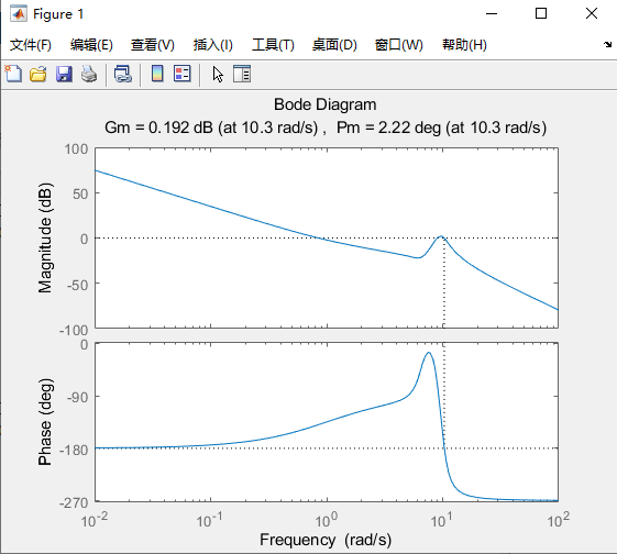
A Bode plot is sufficient to tell you how much margin there is (both phase and gain) before a pole or pole pair in a system crosses the stability boundary -- but it does not, by itself, tell you if the system started out stable.

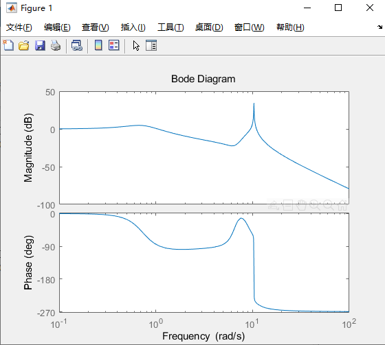
If you start with the prior knowledge that the system was, indeed, stable, then the Bode plot is very useful in determining gain and phase margins, and in tuning the system for better performance from a known stable starting point. This is the case even in the case for a system that starts out with more than 180 degrees of lag, as in the rare but not unheard of case of a type III or higher system.

A Nyquist plot is very handy for telling you whether a system is stable enough, but you still need prior knowledge. In this case, you need to know the number of unstable zeros in the system. I have yet to work on a system where there was any question about this by the time I got to the step of designing a controller, but if I did, I could start with a known-stable system and make a Nyquist plot of it.

Note that if you do have a type III system, or one that has three or more low-frequency poles that you're closing around, then you have at least two gain margins: a low-frequency margin that defines the minimum gain for stability, and a high-frequency one that defines the maximum gain for stability.

TimWescott
  • 2,942
  • 6
  • 13