Determine consecutive occurrences of values

Question

I have a table as shown below:

CAR NAME    INSERT DATE
MERCEDES    2018-01-01
SEAT        2018-01-01
MERCEDES    2018-01-02
BMW         2018-01-02
MERCEDES    2018-01-03
MERCEDES    2018-01-04
MERCEDES    2018-01-05
BMW         2018-01-05
BMW         2018-01-06
SEAT        2018-01-07
BMW         2018-01-08
AUDI        2018-01-08
BMW         2018-01-09  
BMW         2018-01-10
NULL        2018-01-12
SEAT        2018-01-12
SEAT        2018-01-14
SEAT        2018-01-16
BMW         2018-01-17
NULL        2018-01-19 
MERCEDES    2018-01-21
MERCEDES    2018-01-22
MERCEDES    2018-01-23

I would like to know how many consecutive times the same CAR NAME was inserted into the table, when ordered by INSERT DATE, as well as the first and last INSERT DATE. For the purposes of this query, results of one consecutive CAR NAME should be ignored.

For example:

name  count  first     last
mercedes 3 2018-01-03 2018-01-05
bmw      2 2018-01-05 2018-01-06
bmw      2 2018-01-09 2018-01-10
seat     3 2018-01-12 2018-01-16
mercedes 3 2018-01-21 2018-01-23

I have a problem with implementing this, maybe someone could help.

This is for SQL Server. Unfortunately I have only two columns at my disposal.

Answer 1

Your question is not clearly formed, but considering your examples - Phil's comment was correct:

Your example only makes sense if there is another column that defines the order of the data (which is the order you have presented the data as in your question).

Unless you have an additional column with the order of rows - there is no solution to your problem.

Why? Because SQL is based on the theory of relations and in this concept the data itself have no order. So unless you provide an additional column with order of rows (most commonly this would be Id column with incrementing numbers), there would be no way of telling the order of data and thus - your question could not be answered. Without a column with order numbers if you perform SELECT from the database, the SQL officially does not make any guarantees that you will receive rows in the same order every time (and in many cases you won't).

Solution Add another column, e.g. Id as integer and have each row have an incrementing value like this:

Id    NAME         DATE
1   MERCEDES    2018-01-01
2   SEAT        2018-02-01
3   MERCEDES    2018-04-01
4   BMW         2018-01-01
5   MERCEDES    2018-01-01
6   MERCEDES    2018-01-05
7   MERCEDES    2018-01-09

I had much fun figuring out how you could actually query to get the results you wanted, but here it is (sorry I didn't put much time into formatting):

;WITH First (id, car, d, is_first, rn) AS
(
    SELECT *, ROW_NUMBER() OVER (ORDER BY id) rn FROM (
        SELECT
            id
            ,car
            ,d
            ,CASE WHEN ((LEAD(car,1) OVER (ORDER BY id) = car) AND (LAG(car,1) OVER (ORDER BY id) <> car OR LAG(car,1) OVER (ORDER BY id) IS NULL)) THEN 1 ELSE 0 END is_first
        FROM 
            dbo.cars
    ) t
    WHERE t.is_first = 1
),
Last (id, car, d, is_last, rn) AS
(
    SELECT *, ROW_NUMBER() OVER (ORDER BY id) rn FROM (
        SELECT
            id
            ,car
            ,d
            , CASE 
                WHEN (LEAD(car,1) OVER (ORDER BY id) <> car OR LEAD(car,1) OVER (ORDER BY id) IS NULL) AND (LAG(car,1) OVER (ORDER BY id) = car ) THEN 1 ELSE 0 END is_last
        FROM 
            dbo.cars
    ) t
    WHERE t.is_last = 1
)
SELECT
    c.car, COUNT(*) cnt, f.d min_date, l.d max_date
FROM
    First f
    LEFT JOIN Last l ON f.rn = l.rn
    LEFT JOIN cars c ON c.car = f.car AND c.id BETWEEN f.id AND l.id
GROUP BY 
    c.car, f.d, l.d, f.rn
ORDER BY 
    f.rn

The main idea was to find first and last items of ranges (using windowing function LAG and LEAD) and then pair first items with last items using ROW_NUMBER() as keys. And last but not least join these pairs with the original table again just to get COUNT(*)s. Et voila:

Answer 2

Old thread, but it's still an interesting problem.

As Błażej mentioned, we need a column which can be sorted, with no ties. Otherwise, the query will not know which record came first and will count things as a group in some unpredictable way.

Assuming we have this column (let's name it seq), the following query also works:

 WITH grouped_cars AS (
  SELECT name,
         date,
         (
           name,
           -- There is a subtraction below,
           -- don't be fooled by the formatting
           DENSE_RANK() OVER (ORDER BY seq) 
         - DENSE_RANK() OVER (PARTITION BY name ORDER BY seq)
         ) AS car_group
  FROM cars
  )
SELECT MIN(name), -- Could be 'ARBITRARY(name)' in Presto
       COUNT(1) AS count, 
       MIN(date) AS first,
       MAX(date) AS last
FROM grouped_cars
GROUP BY car_group
HAVING COUNT(1) > 1
ORDER BY MIN(date)

Here's a link to the SQLFiddle with the query: http://sqlfiddle.com/#!17/10304/5

The trick is really well explained in this question: Solving "Gaps and Islands" with row_number() and dense_rank()?

How it works?

The trick is that if you subtract two running sequences you get the same number for all elements 8, 9, 10 - 1, 2, 3 = 7, 7, 7. But the result is different if the second sequence is out of order 8, 9, 10, 11, 12 - 1, 2, 3, 1, 2 = 7, 7, 7, 10, 10.

So the first dense_rank() over everything gives you the first running sequence. The second dense_rank() partitioned over the car names gives you the second. When the numbers in it are sequential we have the same result, but every time it "breaks" because another partition is interleaved, the number changes.

Finally, you put the car name together with the number and that gives you something with no real meaning, but that's equal for all items on a sequence with no gaps.

Given that, just group by it and you're done :)

Answer 3

As explained in comments your question is not clear, but if you want, per name, the count, min and max, you can do:

SELECT name, COUNT(*), min(date), max(date) FROM atable GROUP BY name

Try it yourself: http://sqlfiddle.com/#!15/50fcb/5/0

It does not produce the output you show because your example is not clear/complete (example: you list a count of 3 for seat where you have 4 lines of it...)

Answer 4

WITH FIRST1 AS
(   SELECT ID, NAME, DATE1, IS_FIRST,
    ROW_NUMBER() OVER (ORDER BY ID) AS RN 
    FROM
    (   SELECT 
        ID, NAME, DATE1,
        CASE WHEN ( LAG(NAME,1) OVER (ORDER BY ID) <> NAME
                    OR LAG(NAME,1) OVER (ORDER BY ID) IS NULL ) 
                 AND LEAD(NAME,1) OVER (ORDER BY ID) = NAME
            THEN 1 ELSE 0 
        END AS IS_FIRST
        FROM CARS
    ) TEMP1
    WHERE TEMP1.IS_FIRST = 1 ),
LAST1 AS
(   SELECT ID, NAME, DATE1, IS_LAST,
    ROW_NUMBER() OVER (ORDER BY ID) AS RN 
    FROM
    (   SELECT 
        ID, NAME, DATE1,
        CASE WHEN ( LEAD(NAME,1) OVER (ORDER BY ID) <> NAME
                    OR LEAD(NAME,1) OVER (ORDER BY ID) IS NULL ) 
                 AND LAG(NAME,1) OVER (ORDER BY ID) = NAME
            THEN 1 ELSE 0 
        END AS IS_LAST
        FROM CARS
    ) TEMP2 
    WHERE TEMP2.IS_LAST = 1 )
SELECT  
C.NAME, COUNT(*), MIN(F.DATE1), MAX(L.DATE1) 
FROM FIRST1 F 
LEFT JOIN LAST1 L ON F.RN = L.RN
LEFT JOIN CARS C ON C.NAME = F.NAME AND C.ID BETWEEN F.ID AND L.ID
GROUP BY C.NAME, F.DATE1, L.DATE1
ORDER BY F.DATE1; 

Answer 5

<TL;DR>

Definitive answer based on criteria outlined below. The discussion below refers to minor differences in the criteria for the selection of records (don't include NULLs) and their ordering - I finally used the OP's ordering and not the one discussed in the analysis below this section.

SELECT
  name, MAX(rn2) AS cnt, fv_sd, lv_sd
FROM
(
  SELECT
    *, 
    FIRST_VALUE(p_date) OVER (PARTITION BY sd ORDER BY sd) AS fv_sd,
     LAST_VALUE(p_date) OVER (PARTITION BY sd ORDER BY sd) AS lv_sd,
    ROW_NUMBER() OVER (PARTITION BY sd ORDER BY rn) AS rn2
  FROM
  (
    SELECT
      rn, name, lgn, c_diff,  
      SUM(c_diff) OVER (ORDER BY rn, name) AS sd,
      p_date
    FROM
    (
      SELECT 
        rn,
        name, LAG(name) OVER (ORDER BY rn) AS lgn, 
        CASE 
          WHEN name = LAG(name) OVER (ORDER BY rn) 
            THEN 0
            ELSE 1
        END AS c_diff,
        p_date
      FROM test
      -- ORDER BY rn
    ) AS t_01
    -- ORDER BY rn
  ) AS t_02
-- ORDER BY rn
) AS t_03
GROUP BY name, fv_sd, lv_sd
HAVING MAX(rn2) > 1
ORDER BY cnt DESC, fv_sd, lv_sd, name;

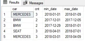
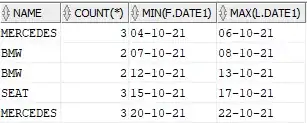
Result (on PostgreSQL and SQL Server):

   name     cnt         fv_sd        lv_sd
MERCEDES      3     2018-01-01  2018-01-09
MERCEDES      3     2018-03-01  2018-04-09
SEAT          3     2018-04-01  2018-07-01
BMW           2     2017-12-01  2017-12-05
BMW           2     2017-12-29  2018-01-01

</TL;DR>

I looked at this and came up with the following solution, which unlike all the others doesn't make use of CTEs. All of the code below can be found on the fiddle here.

My answer is as follows - I'm going to go through my logic, partly to explain it to you, and partly to explain it to myself! :-)

Zeroth Step:

• Right off the bat, we have to decide what we are doing with NULLs in the name field - I've decided to eliminate them - we don't know what they are, and absent any information from the OP, we can only speculate. I therefore will not INSERT records with NULL names.

• I'm using the OP's original INSERTion order - again, absent any other information, we can't know any better!

First step:

I created the table as follows:

CREATE TABLE test
(
  name   VARCHAR (8), 
  p_date DATE
);

using the OP's original data - minus the `NULL's:

INSERT INTO test (name, p_date)
VALUES 
('MERCEDES', '2018-01-01'), 
('SEAT', '2018-02-01'), 
('MERCEDES', '2018-04-01'),
('BMW', '2018-01-01'),
...
... snipped for brevity
...

Second step:

The details from here on differ slightly from the ones outlined in the <TL;DR> definitive section above - the general points about the workings of the SQL still apply - it's just the actual results which differ from above.

Establish an order for the records - this has been pointed out by other posters. I have gone down a different route for numbering - I've used the tuple (date, name) as the ordering criterion - this gives me slightly different results (naturally), but you can adjust this as you will!

SELECT * FROM test ORDER BY p_date, name;

Result:

name    p_date
BMW     2017-01-01
AUDI    2017-12-01
BMW     2017-12-01
SEAT    2017-12-01
BMW     2017-12-05   -- <---  Note the sequence of 5 BMWs.
BMW     2017-12-29
BMW     2018-01-01
BMW     2018-01-01
BMW     2018-01-01
MERCEDES    2018-01-01
...
... snipped for brevity
...

Third step:

SELECT 
  ROW_NUMBER() OVER (ORDER BY p_date, name) AS rn,
  name, LAG(name) OVER (ORDER BY p_date, name), 
  CASE 
    WHEN name = LAG(name) OVER (ORDER BY p_date, name) THEN 0
    ELSE 1
  END AS c_diff,
  p_date
FROM test
ORDER BY p_date;

Result:

rn  name    lag     c_diff      p_date
1   BMW     NULL         1      2017-01-01
2   AUDI    BMW          1      2017-12-01
3   BMW     AUDI         1      2017-12-01
4   SEAT    BMW          1      2017-12-01
5   BMW     SEAT         1      2017-12-05
6   BMW     BMW          0      2017-12-29
7   BMW     BMW          0      2018-01-01

What this does is establish the sequence of records by means of the ROW_NUMBER() function (see the PostgreSQL tutorial here & a more comprehensive list here). Window functions are extremely powerful and well worth putting in the effort to get to know!

So, now we have a rn column associated with our data but there's more to window functions - the LAG() function (see also the related LEAD()) which in conjunction with the CASE expression allows us to start to discriminate between groups of cars. We can see that for every change of car make, there is a 1 and for every time the next car is of the same make as the procediing one, there is a 0.

Step 4:

We use the result of step 3 as a subquery as follows:

SELECT
  rn, name, lgn, c_diff,  
  SUM(c_diff) OVER (ORDER BY rn, name) AS sd,
  p_date
FROM
(
  SELECT 
    ROW_NUMBER() OVER (ORDER BY p_date, name) AS rn,
...
... subquery snipped for brevity
...

Result:

rn  name    lgn     c_diff  sd  p_date
1   BMW         1   1   2017-01-01
2   AUDI    BMW     1   2   2017-12-01
3   BMW     AUDI    1   3   2017-12-01
4   SEAT    BMW     1   4   2017-12-01
5   BMW     SEAT    1   5   2017-12-05  -- <-- note 5
6   BMW     BMW     0   5   2017-12-29  --     "
7   BMW     BMW     0   5   2018-01-01  --     "
...
... results snipped for brevity
...

So, we can see that by taking the cumulative sum, we obtain a way of grouping the cars in the way that we want. We have 5 as the cumulative sum (not related to the fact that there are 5 BMWs - for the 3 Mercs, the cumulative sum is 8).

5th step:

We now establish the first and last dates of sale for the groups of vehicles using the FIRST_VALUE() and LAST_VALUE() window functions (see, they are really important!):

SELECT
  *, -- * is NOT best practice! SQL can be cleaned up here - left for demonstration
  FIRST_VALUE(p_date) OVER (PARTITION BY sd) AS fv_sd,
   LAST_VALUE(p_date) OVER (PARTITION BY sd) AS lv_sd,
   ROW_NUMBER() OVER (PARTITION BY sd ORDER BY rn) AS rn2
FROM
(
  SELECT
    rn, name, lgn, c_diff,
...
... subquery snipped for brevity
...

Results (only shown for the group of 5 BMWs):

rn  name    lgn  c_diff     sd  p_date          fv_sd   lv_sd      rn2
5   BMW     SEAT      1     5   2017-12-05  2017-12-05  2018-01-01  1
6   BMW     BMW       0     5   2017-12-29  2017-12-05  2018-01-01  2
7   BMW     BMW       0     5   2018-01-01  2017-12-05  2018-01-01  3
8   BMW     BMW       0     5   2018-01-01  2017-12-05  2018-01-01  4
9   BMW     BMW       0     5   2018-01-01  2017-12-05  2018-01-01  5

So, we can see that we now have the first date of a purchase for a group and the last date of purchase in a group.

Step 6 (final):

We use the result of Step 5 (again, as a subquery) to get the final result:

SELECT 
  name, MAX(rn2) AS mrn2, fv_sd, lv_sd
FROM
(
  SELECT
    name, rn, p_date,  
    FIRST_VALUE(p_date) OVER (PARTITION BY sd) AS fv_sd,
...
...  subquery snipped for brevity
...

Result (final & full):

    name    mrn2         fv_sd      lv_sd
     BMW       5    2017-12-05  2018-01-01
MERCEDES       2    2018-01-01  2018-01-01
MERCEDES       3    2018-01-05  2018-01-09
    SEAT       2    2018-05-01  2018-07-01

It's not the same as for the others but, as mentioned, I used different ordering criteria for establishing the value of ROW_NUMBER().

Analysis of performance (EXPLAIN (ANALYZE, BUFFERS, VERBOSE) for all:

• the tests were all done using a table sorted on date and name in that order so that the playing field would be level!

My solution:

Planning Time: 0.154 ms
Execution Time: 0.257 ms  -- typical ~ 0.260
54 rows

@Ronie's solution:

Planning Time: 0.134 ms
Execution Time: 0.269 ms  -- typical ~ 0.260
40 rows

@Maheshwaran's solution:

Planning Time: 0.297 ms
Execution Time: 0.379 ms  -- typical ~ .390
78 rows

@BłażejCiesielski's solution:

Planning Time: 0.301 ms
Execution Time: 0.388 ms  -- typical ~ .400
78 rows

I was suprised to see that my solution was as performant as @Ronie's - puzzled, because my EXPLAIN has more steps...

• Obviously a performance analysis based on 23 records on a server over which you have no control is not a great basis for a serious analysis - I would urge anyone undertaking this to do it on their own h/ware with their own normal load.

• Plus, the performance analysis isn't SQL Server. The SQL Server solution is here - I could set up profiling, but it's been a long day! :-)

• it took me a long time to "port" my PostgreSQL solution to SQL Server, but I learnt a lot doing it - about ORDERing and NULLs!

+1 for an interesting question - I learnt a lot! And +1 to @Ronie for a very clever solution!