I am trying to prove with Matlab that if I have an improper system and I place poles at higher and higher frequencies the performances of the system improves. In particular I am considering the following two degree of freedom scheme:
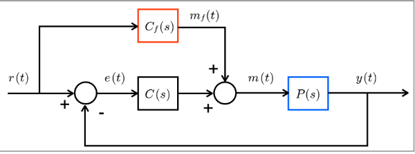
where $C_{f}= \frac{(1+s)(1+0.05s)^{2}]}{(1+\tau s)^{3}}$
My code is the following:
s = tf('s');
P = 1/[(1+s)*(1+0.05*s)^2];
C = (s+1)/s;


tau_1 = 0.1;
CF_1 = [(1+s)*(1+0.05*s)^2]/((1+tau_1*s)^3);

tau_2 = 0.01;
CF_2 = [(1+s)*(1+0.05*s)^2]/((1+tau_2*s)^3);

tau_3 = 0.001;
CF_3 = [(1+s)*(1+0.05*s)^2]/((1+tau_3*s)^3);

T1 = (C+CF_1)*P/(1+P*C);
T2 = (C+CF_2)*P/(1+P*C);
T3 = (C+CF_3)*P/(1+P*C);


figure;
bodemag(T1,'r',T2,'b',T3,'g'),grid
legend('tau = 0.1','tau = 0.01','tau = 0.001')
so what I expected is that the performances with respect to the reference tracking increse as tau gets smaller, but if I do the Bode plot, what I get is:
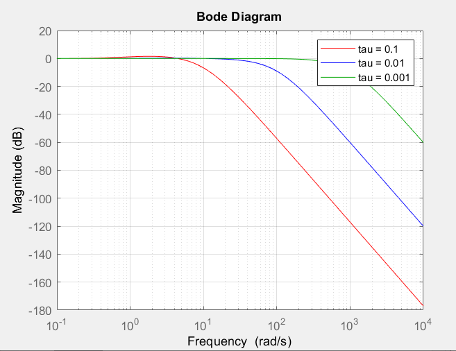
from which I don't really see much of an improvement. Moreover if I change some values:
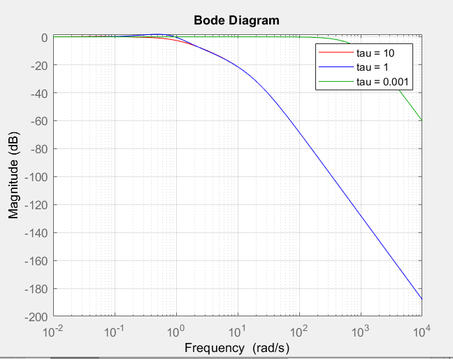
which is somenthing that to me does not makes sense because I should have that with $\tau =1$ I should have better performances than with $\tau =10$, this because with $\tau =1$ the pole is at higher frequencies that with $\tau =10$.
Can somebody please help me solving this problem?
Thanks in advance.
[EDIT] If I plot the step responses I see the same problem:
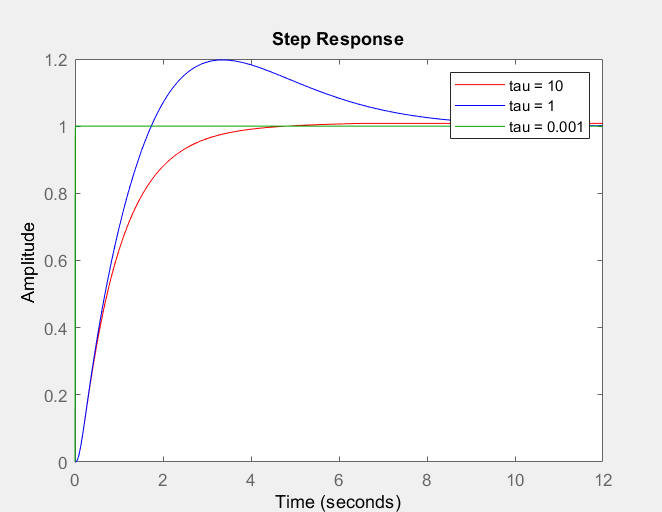
[EDIT 2]For completeness, I post the image of the step response for the first choise of tau's:
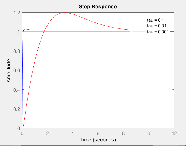
for these values of $\tau$ there is a clear improvement for overshoot and a faster response.
I also tried other values smaller than 1 for $\tau$ and all of these show what I expected in the step response. While for values bigger than 1, I obtain something similar at the other situation.
Does somenone know why this happens? Thanks.
[EDIT 3] With the last one, so values of $\tau$ smaller than 1, I have also noticed an increase in phase margin, so this should mean that the system is performing better.
While, if I consider the values $\tau=1$ $\tau=10$ i get that for the first one the phase margin is 125 deg and for the second is 170 deg. So this should be in according to the fact that $\tau=10$ performs better.