object following using pid

Question

in short, I want to implement a PID controller that takes in distance and returns velocity.

Details: I am simulating robots following each other. I wish to maintain a constant distance, d between these robots. I can obtain the distance between the robots at any time and then I can adjust the velocity of the following robot accordingly. My problem is the formulation that achieves the transformation of the information provided by the PID to velocity so as to achieve this constant distance. My current attempt is to use the error provided by the PID as the velocity for the following robot, that is;

v2 = e(t) where v2 is the velocity of the second/following robot and e(t) is the error yielded by the PID at time t.

The problem with this approach is that it vehicle velocity is only as big as the error, so that way velocity only increases if the error increases, so if the constant distance I want is relatively small. I can never achieve this.

I also tried using the error as the acceleration, with the idea that the velocity should only grow as error grows and decrease in a similar fashion according to:

v2 = v2 + e(t) * dt

where 'dt' is the change in time.

But then when I get negative errors. I wish to avoid reversing or backward motion. So we can call it a stop-go implementation if possible. But ideally when the error in the desired distance reduces ultimately both velocities will be moving with the same velocity. Any approaches and suggestions will be highly appreciated. Thanks very much. I am doing all implementation tests in python. If more clarification is needed please let me know.

score 0 · Answer 1 · answered Apr 29 '21 at 14:05

Let me just reiterate some points that I understood from your problem:

e(t) is the distance from the target distance. So if e(t) = 0.5 and you want to maintain 1m distance b/w robots current distance is 1.5m correct?
You said PID is giving this error which I didn't understand. I believe your approach is correct just needs some corrections.

Instead of using just the error or acceleration you should use both. So you can use this code:

# you need to try different values and tune PID
kp = a 
kd = b
ki = c 
ki_error = 0
# defining a variable to keep error at (t-1) time  
prev_error = 0
def pid_control(e(t)):
    kp_error = kp * e(t)
    kd_error = kd * (e(t) - prev_error)/dt
    ki_error += ki * e(t)
total_error = kp_error + kd_error + ki_error

if total_error &lt; 0 :
     total_error = 0 # for your problem of keeping the car going in reverse

return total_error

Explanation :

kp_error will give higher error (thus higher velocity) the further apart they are
kd_error will give higher error (thus higher velocity) based on how quickly the error increases
ki_error will sum small error and will be able to keep a constant distance no matter how small

The problem with this approach is that it vehicle velocity is only as big as the error, so that way velocity only increases if the error increases, so if the constant distance I want is relatively small. I can never achieve this.

This hopefully will solve your problem if tuned properly. general rule of thumb is kp> kd> ki but feel free to tune further according to your needs.

Pete W · Accepted Answer · 2021-04-30T01:40:56.733

Forget PID at first. If we assume PID, we're skipping steps.

Write down what we know. From your description:

process variable : position
input : (other robot's position - following distance)
loop output : this robot's position
plant input : velocity
plant output : this robot's position
plant dynamics : simple integrator

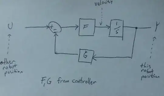
Now we can draw a system diagram:

Note that we left out two very important things: limits on velocity and acceleration. But for now, let's neglect these so we can solve the inside case, when those limits are not reached. In reality, the performance experienced by the user will very much be determined by the edge cases where those limits are in effect.

In a typical PID, G=1 and F = the PID expression.

We can get both stability and zero steady state error for this system with just PI.

A PI controller has a form

F = Kp ( 1 + 1/((Ti)s) ) and G=1

For convenience of analysis, and let's use an alternate form. (The Kp will be different, but no loss of generality. This is still a PI controller)

F = (Kp/s)(1+(Tz)s) and G=1

This form makes the zero in the forward path clearly visible, at s=-1/Tz. The zero in the forward path will remain in the closed loop transfer function, and thus produce step response overshoot, which is not desired per the problem statement.

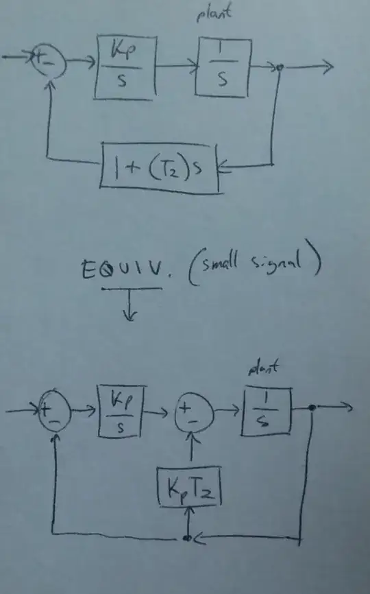
We can get the exact same loop stability by keeping the product FG constant, while eliminating the step response overshoot, (although slower response). Thus we refactor FG into:

F = (Kp/s) and G = (1+(Tz)s)

Now we have deviated from the PI controller, this is slightly different, even though it results in the same stability expression for the complete loop (denominator of closed loop transfer function).

As an optional last step, we can also rearrange the loop into the so-called pseudo-derivative form to get rid of the possibly-troublesome derivative, this rearrangement is shown below.

The rest of the work is about implementing decent saturation and anti-windup logic for the large signal issues. This isn't entirely trivial, and is the real "secret sauce" in some control situations.

object following using pid

2 Answers2

Explanation :