6

According to Hoffman, the standard $k-\epsilon$ turbulence model incorporates a two-layer approach (inner region and outer region formulations to reperesent mixing length) when it comes to regions adjacent to wall surface $(y^+ \approx 30 - 50)$.

My understanding of the $k-\epsilon$ model is that a two additional equations are added to the system of flow governing equations, one equation for kinetic turbulence energy $k$ and the other is for the turbulence energy dissipation rate $\epsilon$, and the closure problem is solved by using dimensionless groups as boundary conditions such as turbulence intensity, turbulence length scale and hydraulic diameter.

My question is why the $k-\epsilon$ model uses zero equations models (algebraic models) for regions adjacent to the wall, what advantages do zero equations models have over $k-\epsilon$ if by definition zero equations models assume that the rate of production of turbulence and the rate of dissipation are approximately equal and they do not include the convection of turbulence?
Algo
  • 2,140
  • 1
  • 20
  • 34

2 Answers2

2

There are two ways of "wall treatment" both feature two layers but at different $y^+$. The general idea is that the velocity gradients in the boundary layer are so high that one would need a very high number of grid cells in order to resolve those gradients. In order to overcome that the flow close to the wall is modeled by one of the following algebraic models (see cfd-online:

  1. Low Reynolds number treatment (LRN)
  2. High Reynolds number treatment (HRN)

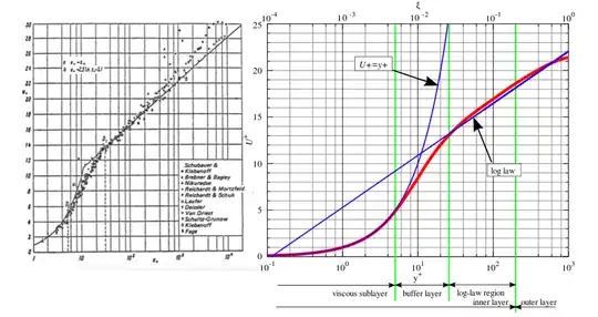
Both treatments are based on the Law of the Wall. Numerous experiments have shown that the boundary layer of a flat plate consists of two distinct regions. From the wall until $y^+ \approx 4$ it is called viscous sublayer with a linear velocity gradient and a logarithmic region from $y^+ \approx 30$. Both layers are joint by a region called buffer-layer.

If one chooses a LRN approach the numerical grid needs to fully resolve the boundary layer in the log-region with (rule of thumb) the first grid-cell at $y^+ =1$. The viscous sub-layer is then modeled algebraically.

In case the HRN approach is chosen the first grid-cell should be in the log-region. Both layers viscous sublayer and log-layer are than modeled algebraically.

enter image description here
from Turbulence and Transport Phenomena by Hanjalic and Wikipedia

The answer to your question has three parts:

  1. Due to the high velocity gradients in the boundary layer it is beneficial with respect to the computational costs to model the flow close to the wall.

  2. The modeling of the boundary layer makes the simulations more robust.

  3. The error introduced into the solution by algebraically modeling the boundary layer is generally small (obviously depending on the simulation itself). Your mentioned neglect of the convective transport of turbulent properties is correct (Which in certain cases will introduce an error).

rul30
  • 1,202
  • 10
  • 24
0

I know that from a CFD point of view (or any time you need a numerical solution to a system of ODEs/PDEs), zero-equation models have two major benefits: 1. they don't need to be integrated by the numerical algorithm, which reduces the computational complexity of the simulation and may improve solution convergence and numerical accuracy, and 2. they don't require any kind of state or history to be maintained (which reduces memory consumption). The cost of this simplicity is, of course, accuracy, especially in regions of high turbulence, flow separation, etc.

Depending on the problem, I usually start with k-e because it's simple and numerically stable, and only after I get a good initial solution and work out all the other bugs in the simulation do I experiment with more complex turbulence models.

Carlton
  • 3,064
  • 2
  • 15
  • 28