A stable transfer function which diverges?

Question

This question might sound stupid as I'm more of a software guy and never really had to do control engineering (besides the 101 classes).

So I have a second order system I could approximate, with the following denominator:

$$s^2 + a_1s + a_0$$

Both $a_1$ and $a_0$ are positive, which means, for a 2^nd order system, that it is stable.

However this system's input is a motor's command (not a speed but a PWM cycle value), and the output is the robots angle.

Technically, my angle will go to $+\infty$ with a constant input, which means my system will never stabilize. So the system should not be stable.

Besides, plotting my transfer function's output to a constant input using scipy gives me the expected result (an angle which ends up growing linearly as the speed stabilizes).

So what am I missing here? Is my model completely wrong? Or did I miss something on the definition of "stability" itself? It would make sense if I worked on the speed but the variable I work on is the angle.

Answer 1

Without any more info, I think your problem arises from the values of $a_0$ and $a_1$. The answer is a little involved, so a bit of systems background is necessary.

The short answer

Your system should be stable, but I don't think you are simulating your system long enough to see it stabilize. Calculate your settling time and simulate it for at least that long to see the complete response transient.

The long answer

The characteristic equation (i.e. denominator of the transfer function) of a general 2nd order system has the following convenient form:

$s^2 + 2 \zeta \omega_n s + w_n^2 $

In this form, $\zeta$ is known as the damping ratio and $\omega_n$ is the natural frequency. As you noted this system is guaranteed to be stable if $w_n^2 > 0$ and $2 \zeta \omega_n > 0$.

In systems engineering we have several rules of thumb for determining the transient response of such systems. One of these is called the settling time $t_s$. It is a measure of how long it takes for the amplitude of the system's oscillations to decrease below a certain threshold, usually 2% or 5% of the steady state value (i.e. the value at which the system stabilizes). You can calculate your settling time using the following approximation (this one is for the 2% criterion):

$t_s = \frac{4}{\zeta \omega_n}$

Therefore, if you do not simulate your system until the settling time, you may see a system that does not appear to stabilize. Note that if $\omega_n$ is very small (therefore your $a_0$ parameter is very small) the settling time could be very long.

For your reference, you can calculate $\omega_n$ and $\zeta$ from your parameters via the following:

$\omega_n = \sqrt{a_0} \qquad \zeta = \frac{a_1}{2 \omega_n}$

A demonstration

Check out what happens when I simulate a second order system with $\omega_n = 0.01$ rad/s and $\zeta = 0.9$ (i.e. $a_0 = 0.0001$ and $a_1 = 0.0180$). Its settling time is approximately 444 seconds. The initial conditions are $\phi = 0$ and $\frac{d\phi}{dt} = 0$. I applied a unit step input (i.e. a constant motor input equal to 1). The following figures show the same system with the exact same conditions, but simulated for different lengths of time. This was all done in MATLAB Simulink, my preferred math simulator.

As you can see in the first image it appears that my system is unstable, but in the second image it becomes clear that it is simply taking a very long time to stabilize.

I hope this helps.

Answer 2

I'm also a software guy and not completely master of the subject, but I tried to model your system. Each step is shown, so you can catch mistakes I did.

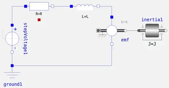
Here is the schematic diagram of DC motor:

Kirchoff's voltage law for electrical circuit: \begin{equation}\label{eq:kirchoff} \tag{1} V_s = V_l + V_r + V_e \\ \end{equation}

Newton's $2^{nd}$ law of motion: \begin{equation}\label{eq:newton} \tag{2} \sum{F} = ma \end{equation}

Equation for Electro-Motive-Force (EMF): \begin{equation}\label{eq:emf} \tag{3} V_e = K_e \dot{\theta} \end{equation}

Equation for electro-mechanical convertion of tourque: \begin{equation}\label{eq:torque} \tag{4} \tau = K_ti \end{equation}

Using equations \ref{eq:kirchoff} & \ref{eq:emf}: $$ u(t) = L \frac{di}{dt} + R i + K_e \dot\theta $$

Using equations \ref{eq:newton} & \ref{eq:torque}: $$ K_t i = J \ddot\theta $$ Laplace transfer of equations: $$ U(s) = s L I(s) + R I(s) + s K_e \Theta(s) \\ K_t I(s) = s^2 J \Theta(s) $$ $I(s)$ is common: $$ I(s) = \frac{U(s) - s K_e \Theta(s)}{s L + R } \\ I(s) = \frac{s^2 J \Theta(s)}{K_t} $$

$$ \frac{U(s) - s K_e \Theta(s)}{s L + R } = \frac{s^2 J \Theta(s)}{K_t} \\ K_t U(s) - s K_t K_e \Theta(s) = s^3 J L \Theta(s) + s^2 J R \Theta(s) \\ K_t U(s) = s^3 J L \Theta(s) + s^2 J R \Theta(s) - s K_t K_e \Theta(s) \\ K_t U(s) = \Theta(s) ( s^3 J L + s^2 J R - s K_t K_e ) $$

Transfer function of system with voltage input and position output: $$ \frac{\Theta(s)}{U(s)} = \frac{K_t}{s^3 J L + s^2 J R - s K_t K_e} $$

If we want to investigate voltage-speed relationship: $$ s(\frac{\Theta(s)}{U(s)}) = s(\frac{K_t}{s^3 J L + s^2 J R - s K_t K_e}) \\ \frac{s\Theta(s)}{U(s)} = \frac{K_t}{s^2 J L + s J R - K_t K_e}) $$

Applying step input, which is PWM with 100% duty cycle: $$ \Theta(s) = \frac{\alpha}{s} \frac{K_t}{(s^3 J L + s^2 J R - s K_t K_e)} $$

It might be good to investigate stability of a system with impulse input instead of step input.

With mobility analogy, Voltage & Velocity are cross variables, Current & Force are through variables, you can also investigate the system as RLC series circuit as shown below.

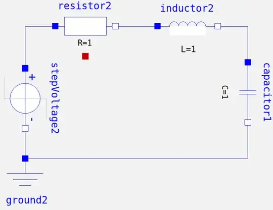
For $u(t)$ input $V_c$ output, it is voltage-velocity relation and $u(t)$ input $\int{v_c(t)dt}$ for voltage-position relation. So it adds 1 more degree to your system.